SeisSol Performance and Scalability with Cornelis Networks Omni-Path on 3rd Generation Intel Xeon Scalable Processors

Cornelis NetworksTM is the leading independent provider of purpose-built, open-source, scale-out interconnects for high-performance computing, artificial intelligence, and data analytics. The Cornelis Networks Omni-Path high-performance networking fabric delivers class-leading message rate, latency, and scalability allowing customers to deploy solutions which enable faster time to solution and improved workload scalability combined with leading price/performance. To highlight the capabilities of the Omni-Path fabric, this paper analyzes the performance of an industry standard SeisSol (www.seissol.org) benchmark case on a 3rd Generation Intel® Xeon® Scalable processor-based cluster.
In this article, a well-known benchmark is decomposed into three different resolutions, and scaling studies are performed using up to 32 dual-socket Intel Xeon Platinum 8358 nodes. Performance is studied in terms of job throughput (cases per day), effective CPU utilization (GFLOPS), and the standard deviation of these performance measurements. MPI profiling is performed to understand the content of the MPI messaging in SeisSol and potential performance optimizations. Lastly, helpful tips for compiling and running SeisSol based on Cornelis Networks experiences are provided.
Problem Statement and Setup
SeisSol is a high performance, open-source seismic wave simulation software package used in geophysics academia1 and may be applied in the oil and gas industries. Using a hybrid OpenMP/MPI version of SeisSol v1.0.1, Cornelis Networks conducted an investigation of the TPV332 benchmark which models the behavior of a spontaneous rupture on a vertical strike slip fault with a low velocity fault zone. Initial normal stresses are constant while the shear stresses gradually decrease to prevent spontaneous rupture from extending beyond the fault’s boundaries. The model excludes gravitational forces. Nucleation is initiated by applying additional shear stress within 550 meters of the hypocenter, where the initial shear stress slightly surpasses the yield stress tapering down to the background level between 550 meters and 800 meters of the hypocenter.3
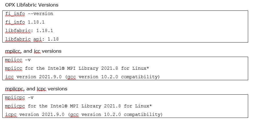
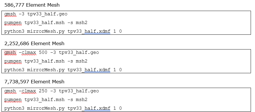
To study scaling efficiencies, MPI communications, and performance statistics, the TPV33 benchmark was meshed using approximately 0.58M, 2.2M, and 7.7M elements. Gmsh-4.11.1 is used to partition the domain,4 with the number of elements controlled with the clmax flag. The Intel MPI Library 2021.10 is used. Static core-thread affinity is set by exporting OMP_PROC_BIND=true. The SeiSol documentation suggests leaving one core per rank dedicated for communication which should improve performance. This can be accomplished by specifying OMP_NUM_THREADS=7 and I_MPI_PIN_DOMAIN=8:compact. This decomposition was found to be most optimal on the dual-socket 32-core Intel Xeon Platinum 8358 nodes (64 total cores per node). The highly optimized Cornelis Omni-Path Express (OPX) libfabric provider version 1.18.1 is used,5 and an example of a job submission script and mpirun command is shown in a later section.
Figure 1 presents a graphical representation of the transient normal stresses at the model’s surface – visualization of the benchmark output was first performed to ensure the accuracy of the simulations before successive benchmarking.
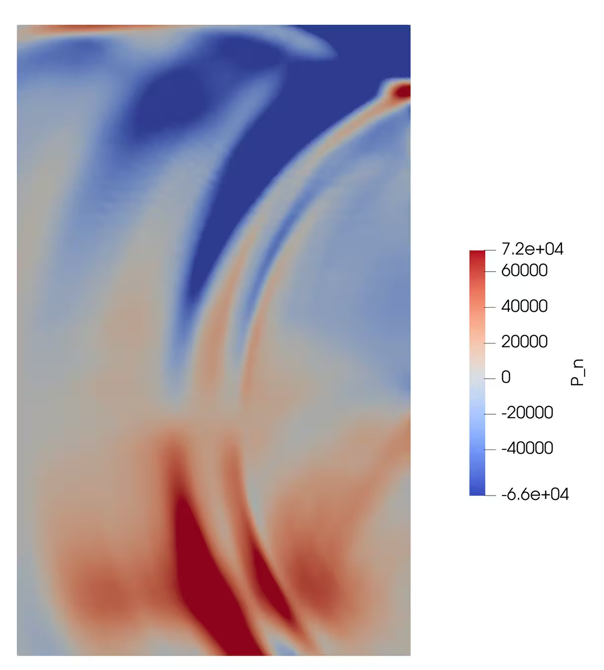
Figure 1: Visualization of transient normal stresses at models surface for TPV33 simulation.
Scalability
Simulations are run on up to 32 dual-socket Intel Xeon Scalable Platinum 8358 nodes. Each node contains 4 NUMA nodes of 16 cores each, for a total of up to 2048 cores. The nodes are interconnected with Cornelis Networks Omni-Path 100Gbps network fabric.
To gauge scalability, SeisSol’s developers recommend reporting the number of GFLOPS normalized by the node count. Here, GFLOPS is defined as the number of operations executed by the compute kernels,6 and is reported as [Total calculated HW-GFLOP/s], at the end of the simulation. Normalization of the performance by the respective node count is abstained to better provide insights into the effective utilization of computational resources used by the simulations, enable analysis of scaling efficiencies across different meshes, and to get a clearer picture of any run-to-run variability.
To analyze the speedup of these simulations, job throughput – defined as the number of simulations completed per day – is computed. This is accomplished by dividing the amount of time in a day by the simulation time. In a perfect compute environment, job throughput and GFLOPS are expected to scale linearly with respect to node count and are therefore chosen as performance metrics. Simulations are run five times for each mesh resolution, and results are averaged and plotted in Figure 2.
As shown in Figure 2, the 0.58M element mesh 32 node simulations averaged a job throughput of 533 cases per day, whereas single node simulations with the same mesh yielded 39 cases per day. This corresponds to a scaling efficiency of about 42.3%. Similar analysis for simulations using 2.2M and 7.6M elements results in scaling efficiencies of 70.8% and 82.8% respectively. The higher resolution meshes have a better scaling efficiency because the ratio of compute to communication is higher.
Overall, there is a 1.92X increase in GFLOPS for 32 node simulations when increasing from the 0.58M element mesh to the 7.6M element mesh. The finest mesh achieved a performance of 30640 GFLOPS for 32 node simulations and 1148 GFLOPS for single node simulations yielding a scaling efficiency of 83.3%. Corresponding analysis for 0.58M and 2.2M element simulations results in scaling efficiencies of 43.3% and 60.3% respectively.
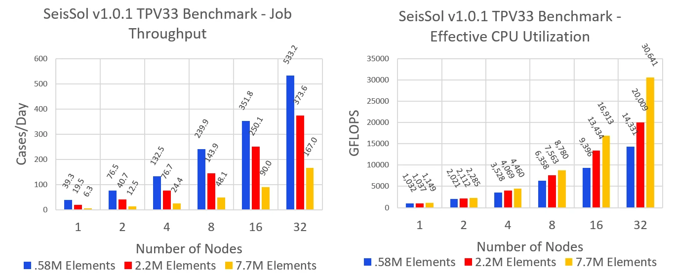
Figure 2: Averaged results for job throughput (Left) and effective CPU utilization (Right) for TPV33 simulations using meshes consisting of 0.58, 2.2, and 7.6 million elements executed on Intel Xeon Scalable Platinum 8358 dual-socket cores.
Ultimately, low-resolution simulations enable faster turnaround time, while high resolution simulations make more effective use of computational resources and reduce run to run variability, potentially allowing for more careful tuning studies and conclusive behavior. Increasing node count leads to a corresponding rise in the variability across simulations. To visualize this trend, Figure 3 displays the relative standard deviation (RSD) for job throughput and GFLOPS. The RSD is a measure of run-to-run variation for these performance metrics.
Figure 3 suggests mesh resolution is correlated to the RSD. In general, the RSD for both job throughput and GFLOPS increases with increasing node count. In particular 0.58M element, TPV33 simulations using eight nodes and greater result in a job throughput RSD greater than 5%. Given such a substantial performance variability, remarks on future optimization studies incorporating variations in MPI, fabric provider, and tunings would be inconclusive. To address this concern a 7.7M element mesh can be used instead. 7.7M element TPV33 simulations result in an RSD close to 1% for both job throughput and GFLOPS across all node counts with the exception of 16 node runs. Any performance tuning which has a performance impact above the RSD could be considered significant.
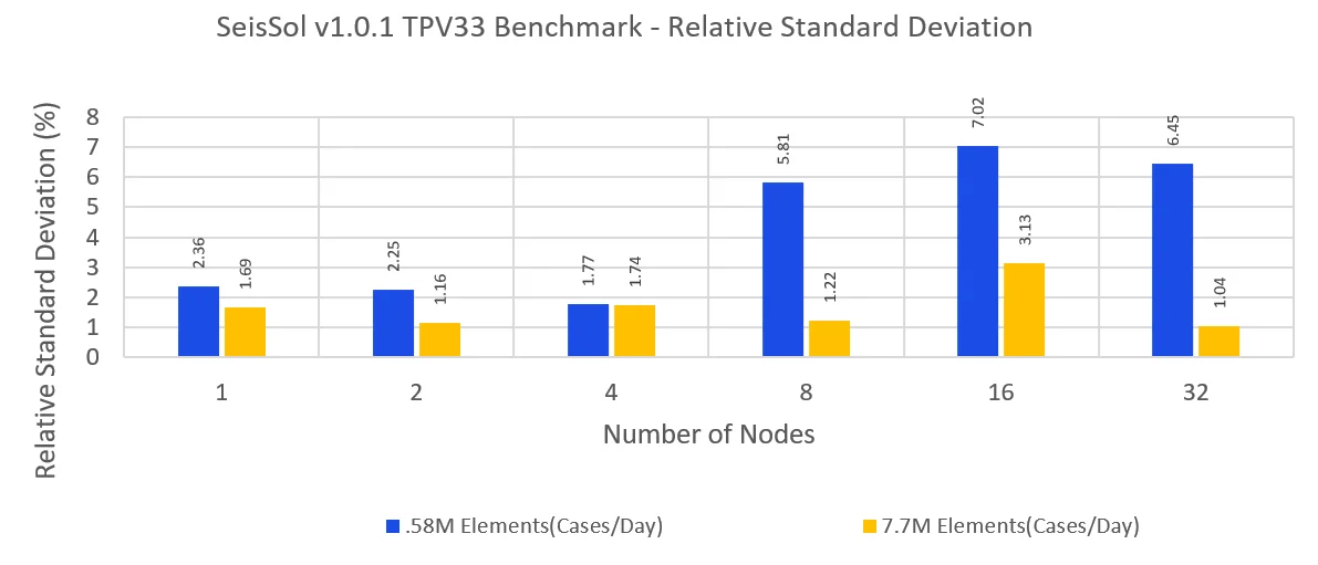
Figure 3: Relative standard deviation of GFLOPS and job throughput for TPV33 simulations using 0.58 and 7.7 million elements for 1,2,4,8,16, and 32 nodes.
MPI Communications
MPI communications are assessed with Intel’s Application Performance Snapshot (APS).7 Care was taken to maximize the performance metrics when selecting the hybrid MPI/OpenMPI decomposition. It was found that using seven OpenMP threads per rank, and one dedicated core for communication, while binding the threads to the cores led to a consistent CPU utilization of 700%-800% per rank. Consequently, APS reported that the binding scheme used leads to an OpenMP imbalance between only 2%-3%, independent of the mesh size and node count.
Denote MPI time as the total amount of simulation time spent calling MPI functions. Approximately 50% to 70% at 1 node to 32 nodes, respectively, of the simulation time is consumed by the MPI functions. While this might indicate a high MPI imbalance with the potential for tuning, between 60%-90% of the MPI time is spent in MPI_Test. The dedicated communication core in SeisSol runs MPI_Test in an infinite loop to ensure MPI progress while the simulation is running. To better visualize our findings, the percent time spent calling these MPI functions is plotted as a pie chart in Figure 4. APP_TIME in Figure 4 denotes the percent time spent outside of MPI function calls, and OTHER are a consortium of negligible MPI function calls for the given simulation.
Here, percent time refers to the wall clock time spent calling any of the aforementioned categories over the total simulation time. Neglecting MPI_Test and APP_TIME for brevity, it is apparent that simulations spend most of their time calling Allreduce. This time percentage decreases with increasing mesh resolution and in general lower resolution simulations will result in simulations spending more proportional time executing MPI functions. Moreover, it is observed that increasing the number of allocated nodes for a simulation results in an increase in the percent time calling Allreduce. In particular for 2.2M element simulations, the percent time increases from 2.35% for single node runs to 22% with 32 nodes runs. Intuitively this makes sense as there is an increase in ranks, and an increase in inter-node communications for these simulations.
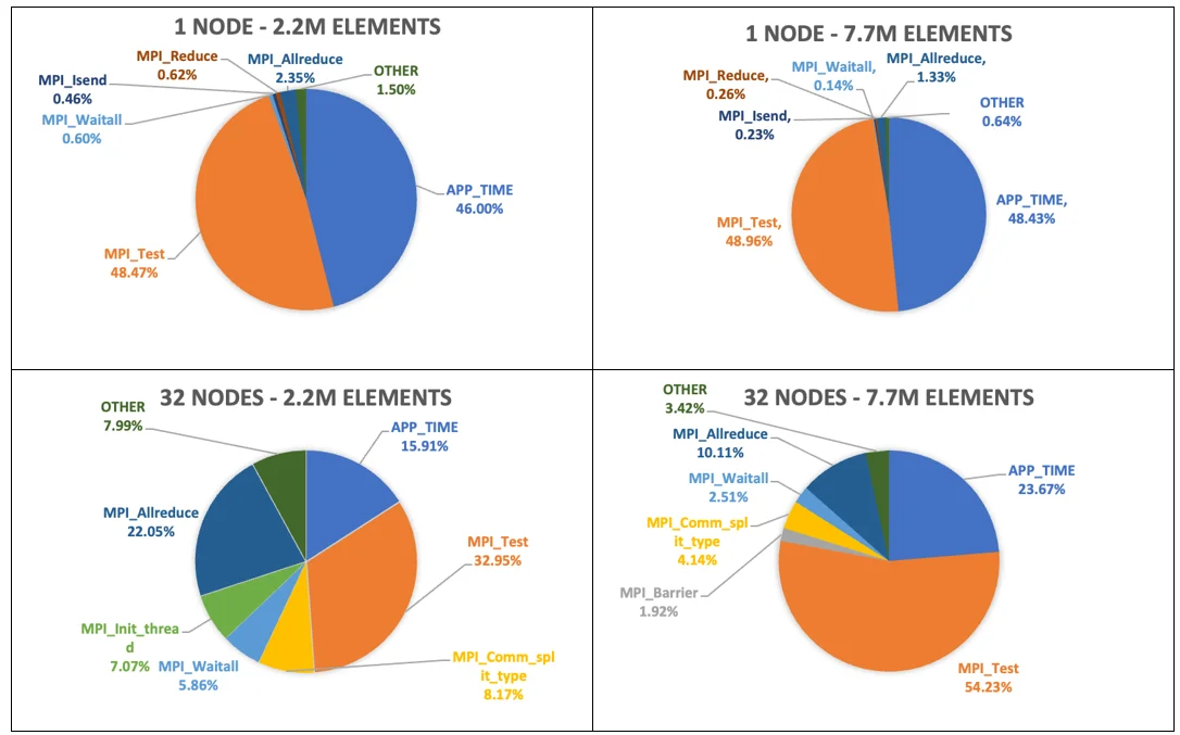
Figure 4: MPI Profiles for SeisSol TPV33 benchmark.
Based on Figure 4, it appears that SeisSol could gain performance improvements by optimizing Allreduce. One approach involves leveraging APS to identify the message sizes Allreduce spends the most time on. After analyzing the message sizes, adjustments can be made to tailor the algorithm used by Allreduce to better suit these message sizes. However, it’s important to note that Allreduce can serve to synchronize application state, similar to a Barrier. The Allreduce operation cannot begin until all ranks reach this point in the code – if Allreduce is instead acting like a Barrier before the Allreduce message passing begins, any algorithm adjustments might not have a significant impact on the Allreduce time. To explore this idea, SeisSol was recompiled with an artificially inserted Barrier before every Allreduce function call. It was found that the proportion of MPI time spent on Allreduce decreased significantly to below 0.1% and the expensive MPI function moved to the Barrier. This implies that Allreduce acts more like an application synchronization function compensating for compute imbalances, and algorithm adjustments would likely not increase performance.
Compiling and Running SeisSol
To compile SeisSol-v1.0.1, we follow the build instructions8 with slight modifications to take advantage of Intel oneAPI MKL’s, BLAS, and SCALAPACK libraries. The GEMM tools libxsmm and PSpaMM are used for matrix operations because they perform better on smaller matrices than BLAS. BLAS is only used for the Eigen dependency. It is recommended to read about the Command-Line-
Link Tool9 to better customize the build for the mpi/compiler of your choice. SeisSol is compiled using Intel C++ Compiler Classic along with the Intel MPI library, mpiicpc/mpiicc version 2021.10.0, and icpc/icc version 2021.9.0.10
SeisSol’s dependencies mainly use CMake for the build process which includes modules FindBLAS and FindLAPACK. If MKL is sourced correctly, the BLAS/LAPACK libraries and linker flags should be set appropriately. Trouble can occur during the build process if dependency installations are in non-standard locations. Using MKL’s link tool, BLAS_LIBRARIES, BLAS_LINKER_FLAGS, LAPACK_LIBRARIES, and LAPACK_LINKER FLAGS can be exported manually and cmake should be able to detect them automatically.
If libraries are not linking properly it is recommended to go through the generated CMakeCache.txt and specify libraries and include directories on the command line. If dependencies are in non-standard locations, appending their installation prefixes to CMAKE_PREFIX_PATH can help cmake find libraries and header files.
There were some API changes from when SeisSol last updated their documentation for the latest hdf5 library version 1.14.0. This can error out the cmake process. To work around these API changes, configuring hdf5 using the following command will switch the API to a SeisSol-v1.0.1 compliant version.

When building PUMGen11 the following CMake Error is encountered:

This originates from the set_target_properties line in the following CMakeList.txt snippet:

The error is resolved by enclosing ${INSTALL_RPATH} in quotes as show below:

This fix has been reported and merged into the master branch of PUMgen.12 A sample SLURM submission script is provided below for SeisSol TPV33 simulations:
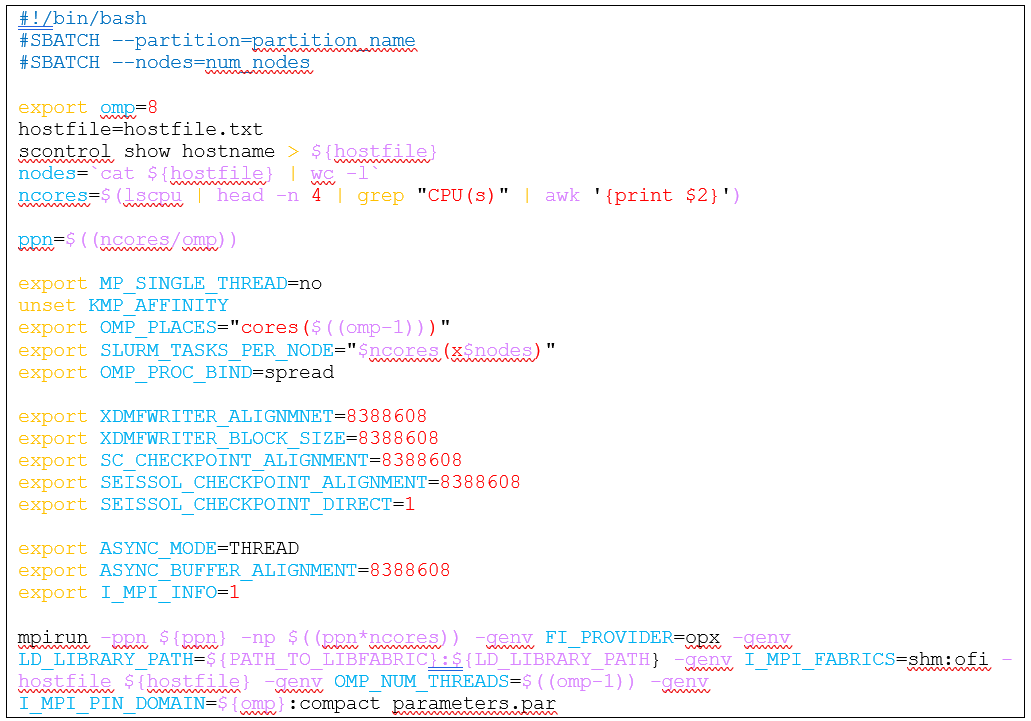
Provided that the current working directory holds the necessary inputs, the submission script should execute SeisSol. The variable omp can be toggled and the number of cores per rank and processes per node will be adjusted accordingly. It is important that omp is a divisor of the number of cores per node to make use of all computational resources.
Conclusions
This study led to a general build recipe, and analytic pipeline to evaluate SeisSol’s performance in different contexts. Results show SeisSol’s potential for use in academic and industry settings. Low resolution meshes are useful in settings that require a high job throughput, while high resolution meshes yield better statistics and GFLOPS at the cost of job throughput. Analysis of MPI communications suggests that Allreduce algorithm tuning will not lead to a substantial increase in performance. Future optimization studies will focus on point-to-point communications and potential optimizations over Cornelis Omni-Path.
System Configuration
Simulations performed on 2 socket Intel Xeon Scalable Platinum 8358 Processor-based servers. Rocky Linux 8.4 (Green Obsidian). 4.18.0-305.19.1.el8_4.x86_64 kernel. 32x16GB, 256 GB total, 3200 MT/s. BIOS: Hyper-Threading: Disabled. Virtualization Technology: Disabled. Power and Performance Policy: Performance. C-State: C0/C1. C6: Disabled. P-States: Disabled. Turbo Boost: Enabled.
Legal Disclaimer
You may not use or facilitate the use of this document in connection with any infringement or other legal analysis concerning Cornelis Networks products described herein. You agree to grant Cornelis Networks a non-exclusive, royalty-free license to any patent claim thereafter drafted which includes subject matter disclosed herein.
No license (express or implied, by estoppel or otherwise) to any intellectual property rights is granted by this document.
All product plans and roadmaps are subject to change without notice.
The products described may contain design defects or errors known as errata which may cause the product to deviate from published specifications. Current characterized errata are available on request.
Cornelis Networks technologies may require enabled hardware, software, or service activation.
No product or component can be absolutely secure.
Your costs and results may vary.
Cornelis, Cornelis Networks, Omni-Path, Omni-Path Express, and the Cornelis Networks logo belong to Cornelis Networks, Inc. Other names and brands may be claimed as the property of others.
Copyright © 2024, Cornelis Networks, Inc. All rights reserved.
References
- https://doi.org/10.1126/science.adi0685
- https://github.com/SeisSol/Examples/tree/master/tpv33
- https://strike.scec.org/cvws/download/TPV33_Description_v04.pdf
- https://seissol.readthedocs/io/en/latest/gmsh.html
- https://github.com/ofiwg/libfabric/tree/v1.18.1
- https://buildmedia.readthedocs.org/media/pdf/seissol/latest/seissol.pdf
- https://www.intel.com/content/www/us/en/developer/tools/oneapi/toolkits.html#gs.0o6ces
- https://seissol.readthedocs.io/en/latest/installing-dependencies.html
- https://www.intel.com/content/www/us/en/docs/onemkl/developer-guide-linux/2023-0/using-the-command-line-link-tool.html
- https://www.intel.com/content/www/us/en/developer/tools/oneapi/overview.html
- https://github.com/SeisSol/PUMGen
- https://github.com/SeisSol/PUMGen/pull/66